ROC and PR curves are commonly used to present results for binary decision problems in machine learning. The ROC curve is created by plotting the true positive rate (TPR) against the false positive rate (FPR) at various threshold settings. Each point of the ROC curve (i.e. threshold) corresponds to specific values of sensitivity and specificity. The area under the ROC curve (AUC) is a summary measure of performance that indicates whether on average a true positive is ranked higher than a false positives. If model A has higher AUC than model B, model A is performing better on average, but there still could be specific areas of the ROC space where model B is better (i.e. thresholds for which sensitivity and specificity are higher for model B than A. However, when dealing with highly skewed datasets, Precision-Recall (PR) curves give a more informative picture of an algorithm's performance. There is deep connection between ROC space and PR space, such that a curve dominates in ROC space if and only if it dominates in PR space. The precision-recall curve shows the tradeoff between precision and recall for different threshold. A high area under the curve represents both high recall and high precision, where high precision, x-axis, relates to a low false positive rate, and high recall, y-axis, relates to a low false negative rate. High scores for both show that the classifier is returning accurate results (high precision), as well as returning a majority of all positive results (high recall).
Sensitivity (positive in disease)
Sensitivity is the ability of a test to correctly classify an individual as ′diseased′
Sensitivity = a / a+c
= a (true positive) / a+c (true positive + false negative)
= Probability of being test positive when disease present.
Specificity (negative in health)
The ability of a test to correctly classify an individual as disease- free is called the test′s specificity
Specificity = d / b+d
= d (true negative) / b+d (true negative + false positive)
= Probability of being test negative when disease absent.
Sensitivity and specificity are inversely proportional, meaning that as the sensitivity increases, the specificity decreases and vice versa.
Positive Predictive Value (PPV)
It is the percentage of patients with a positive test who actually have the disease.
PPV: = a / a+b
= a (true positive) / a+b (true positive + false positive)
= Probability (patient having disease when test is positive)
Negative Predictive Value (NPV)
It is the percentage of patients with a negative test who do not have the disease.
NPV:    =   d / c+d
=   d (true negative) / c+d (false negative + true negative)
=   Probability (patient not having disease when test is negative)
Positive and negative predictive values are influenced by the prevalence of disease in the population that is being tested. If we test in a high prevalence setting, it is more likely that persons who test positive truly have disease than if the test is performed in a population with low prevalence. So the PPV will increase with increasing prevalence and NPV decreases with increase in prevalence.
Methods to find the ‘optimal’ threshold point
Three criteria are used to find optimal threshold point from ROC curve. These criteria are known as points on curve closest to the (0, 1), Youden index, and minimize cost criterion. First two methods give equal weight to sensitivity and specificity and impose no ethical, cost, and no prevalence constraints. The third criterion considers cost which mainly includes financial cost for correct and false diagnosis, cost of discomfort to person caused by treatment, and cost of further investigation when needed. This method is rarely used in medical literature because it is difficult to estimate the respective costs and prevalence is often difficult to assess.
Youden index is more commonly used criterion because this index reflects the intension to maximize the correct classification rate and is easy to calculate. It maximizes the vertical distance from line of equality to the point [x, y] as shown in Figure. The x represents (1-specificity) and y represents sensitivity. In other words, the Youden index J is the point on the ROC curve which is farthest from line of equality (diagonal line). The main aim of Youden index is to maximize the difference between TPR (sensitivity) and FPR (1 –specificty) and little algebra yields J = max[sensitivity+specificty]. The value of J for continuous test can be located by doing a search of plausible values where sum of sensitivity and specificity can be maximum:
j= model_metric['thres'].iloc[model_metric['yod_index'].idxmax()-1]
Sometimes a second cutoff that is bigger than j but less than 1 is needed. This cutoff can be used to stratify the positively predicted values to moderate and high prediction for example(needed for risk prediction stratification). This cutoff can be calculated using the accuracy measurement using the following method:
cutoff2=cu.cal_cutoff2(model_metric)
with
def cal_cutoff2(data):
    val=0
    for i in range(len(data)-10):
    if((abs(data['acc'].iloc[i]-data['acc'].iloc[i+10]))<0.002):
        val=data['thres'].iloc[i]
        break
    return(val)
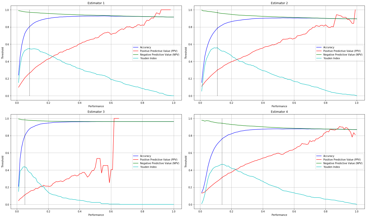
The chart bellow illustrates the relationship between the different performance metrics ( prevalence is exluded) in an example of 4 estimators apllied on 4 -classes data
Calculation of performance metrics
Here is the python code for the calculation of performance metrics
def calculate_metric(outcome, score):
    obser = np.zeros(len(outcome))
    obser[[i for i, x in enumerate(outcome) if x == 1 ]] = 1 ;
    obser = [float(i) for i in obser]
    score = [float(i) for i in score]
    prev = round(sum(obser)/len(obser),2)
    thres = np.arange(0.01,1.01,0.01)#(0.01,0.98,0.01)
    xval = thres
    acc = np.zeros(len(thres))
    ppv = np.zeros(len(thres))
    npv = np.zeros(len(thres))
    sen = np.zeros(len(thres))
    spe = np.zeros(len(thres))
    yod = np.zeros(len(thres))
    auc = np.zeros(len(thres))
    recall = np.zeros(len(thres))
    precision = np.zeros(len(thres))
    F1 = np.zeros(len(thres))
    for l in range(len(thres)):
        plotdata = ROC_parameters(obser,score,thres[l])
        acc[l] = round(plotdata[0],3)
        ppv[l] = round(plotdata[1],3)
        npv[l] = round(plotdata[2],3)
        sen[l] = round(plotdata[3],3)
        spe[l] = round(plotdata[4],3)
        yod[l] = round(plotdata[5],3)
        recall[l] = round(plotdata[6],3)
        precision[l] = round(plotdata[7],3)
        F1[l] = round(plotdata[8],3)
        auc[l] = roc_auc_score(obser, score)
    prev = round(sum(obser)/len(obser),2)
    #roc_vals=np.zeros((length(spe),8))
    roc_vals=pd.DataFrame(index=range(1,101), columns=[["thres","acc","ppv","npv","specificity","sensitivity","yod_index","recall","precision","F1","auc"]])
    #roc_vals <- dacolnames(roc_vals) <- c("thres","acc","ppv","npv","specificity","sensitivity","yod_index","auc")
    roc_vals['thres']=thres
    roc_vals['acc']= acc
    roc_vals['ppv'] = ppv
    roc_vals['npv'] = npv
    roc_vals['specificity'] =spe
    roc_vals['sensitivity'] = sen
    roc_vals['yod_index'] = yod;
    roc_vals['recall'] = recall;
    roc_vals['precision'] = precision
    roc_vals['F1'] = F1;
    roc_vals['auc'] = auc;
    return roc_vals

def ROC_parameters(obser,score,thr):
    #print obser,score,thr
    temp=np.zeros(len(score))
    #print thr;
    temp[[ i for i, x in enumerate(score) if x >= thr ]]= 1
    p_ind=[ i for i, x in enumerate(obser) if x == 1 ]
    n_ind = [ i for i, x in enumerate(obser) if x == 0 ]
    TP = sum(temp[p_ind]==1)
    FP = sum(temp[n_ind]==1)
    TN =sum(temp[n_ind]==0)
    FN = sum(temp[p_ind]==0)
    acc = (float)(TP+TN)/len(temp)
    recall=0
    precision=0
    #print TP,FP,TN,FN;
    if TP+FP>0:
        ppv = (float)(TP)/(TP+FP)
    else:
        ppv=np.NaN
    if TN+FN>0:
        npv = (float)(TN)/(TN+FN)
    else:
        npv=np.NaN
    if TP+FN>0:
        sen = (float)(TP)/(TP+FN)
    else:
        sen=np.NaN
    if TN+FP>0:
        spe = (float)(TN)/(TN+FP)
    else:
        spe=np.NaN
    if TP+FN>0:
        recall = (float)(TP)/(TP+FN)
    else:
        recall=np.NaN
    if TP+FP>0:
        precision = (float)(TP)/(TP+FP)
    else:
        precision=np.NaN
    if recall+precision>0:
        F1 = (float)((2*recall*precision)/(recall+precision))
    else:
        F1=np.NaN
    yod = (float)(sen+spe-1)
    ls=list();
    ls.append(acc)
    ls.append(ppv)
    ls.append(npv)
    ls.append(sen)
    ls.append(spe)
    ls.append(yod)
    ls.append(recall)
    ls.append(precision)
    ls.append(F1)
    return ls
calculating performance measurements and confidence intervals using Boostraping
def calculate_metric_boostrap(outcome, score):
    d = []
    for p in range(0,len(score)):
        d.append((score[p]))
    score=pd.Series(d)
    n_bootstraps = 0
    rng_seed = 42  # control reproducibility
    scores_table = {}
    rng = np.random.RandomState(rng_seed)
    for i in range(n_bootstraps):
    # bootstrap by sampling with replacement on the prediction indices
        indices = rng.random_integers(0, len(outcome) - 1, len(outcome))
        if len(np.unique(outcome[indices])) < 2:
        # We need at least one positive and one negative sample for ROC AUC
        # to be defined: reject the sample
            continue
        scores_table[i]= calculate_metric(outcome[indices], score[indices])

    panel = pd.Panel(scores_table)
    df=panel.mean(axis=0)
    return df,panel

def confidence_interval(panel):
    vector = []
    confidence_lower=panel[1].copy()
    confidence_upper=panel[1].copy()
    nr=len(panel[1].axes[0])
    nc=len(panel[1].axes[1])
    for ix in  range(0,nr):
        for iy in range(0,nc):
            vector = []
            for k, df in panel.iteritems():
                vector.append(df.iloc[ix,iy])
            sorted_vector = np.array(vector)
            sorted_vector.sort()
            confidence_lower.iloc[ix,iy] = sorted_vector[int(0.05 * len(sorted_vector))]
            confidence_upper.iloc[ix,iy] = sorted_vector[int(0.95 * len(sorted_vector))]
    return confidence_lower, confidence_upper
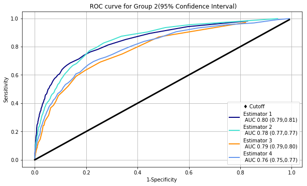
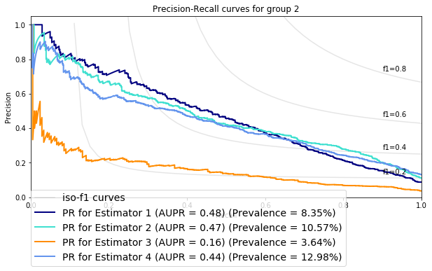
The chart bellow illustrates ROC and PR curves for 4 different estimators applied on the same data
 The performances of the algorithms appear to be comparable in ROC space, however, in PR space we can see that Estimator 4 has a clear advantage over Estimator 3.